7.1 Refresher - standard R plotting functions
7.1.1 Plot() function
plot() can be used for several other applications. These include line graphs (showing, for example, changes over time) and volcano plots (for gene expression analysis). Let’s revisit this using our beaver temperature dataset, and preparing a scatterplot of our time-merged data.
-
Make a scatterplot comparing body temperature of the two beavers from our merged data.frame.
-
Review the
plotdocumentation to add the following:- a title to the plot,
-
replace the axis names with
Beaver 1andBeaver 2 - change the plot symbols
- add a trend line
This gives us a correlation, but does not show how data changes over time. For this we need a different type of plot, either type = "l", which gives a line plot; or type = "o", which standard for overplot and gives points connected by lines. Drawing this plot is a little more involved, since we need to plot the two datasets separately, both scaled against time.
Before we start anything we need to know the maximum range required for the axes. By default, when we plot the graph, it will scale for the first animal, but adding others may go outside the display range
temp.range <- range(beaver.temp$temp.x, beaver.temp$temp.y, na.rm = TRUE)

# Set up the plot for the first animal
# In this case, we'll define the axis labels at the outset
# xaxt = 'n' means not to give the x-axis scale - we'll add that in a moment
plot(beaver.temp$temp.x, type="o", col="blue",
     ylim = temp.range, xaxt = 'n',
     xlab = "Time", ylab="Temp")

# Now add the second animal data
lines(beaver.temp$temp.y, type = "o", col="red")

axis(1, at = 3+6*c(0:19), lab = beaver.temp$time[3+6*c(0:19)])
title(main="Diurnal temperature variation")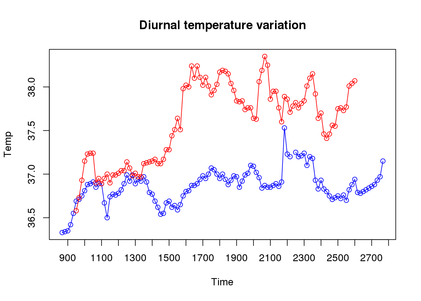
(Optional)
Further timecourse plotting practice
-
Using another built-in R dataset
Indometh, examine the dataset and plot time course changes for two or more of the six samples. -
Give each sample a different colour.
-
Try to label and scale the axes appropriately.
7.1.2 Boxplots
Let’s plot our microarray data from the previous exercise side by side to show the unnormalised data alongside the normalised dataset. The red squares on each boxplot shows the location of the mean value.
par(mfrow=c(1,2))
means <- colMeans(golub.log)
boxplot(golub.log[,1:15],las=2,main="Log10 transformed")
points(1:15, means[1:15], pch=15, col='red')

means <- colMeans(golub.norm)
boxplot(golub.norm[,1:15],las=2,main="Normalised expression")
points(1:15, means[1:15], pch=15, col='red')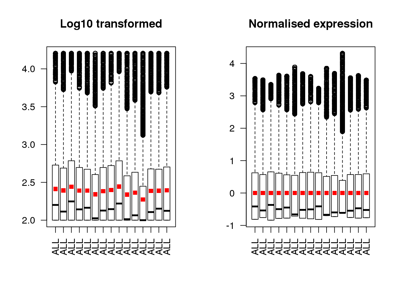
Make the y-axes to be the same range in both plots so that it is not misleading.
7.1.3 Heatmaps
Another commonly used way of displaying biological datasets is the heatmap. This is commonly used for gene expression analysis, but it can be used for any dataset where multiple quantitative measurements are carried out on several samples. Not only can an R-generated heatmap help in the visualisation of these sort of datasets, but the heatmap command can also be used to automatically organise samples and/or measurements into dendrograms, showing the similarity relationship between them.
For a first example, let’s plot a heatmap for our 100 key Golub dataset genes.
# Run the simplest heatmap, with all default settings
heatmap(golub.100)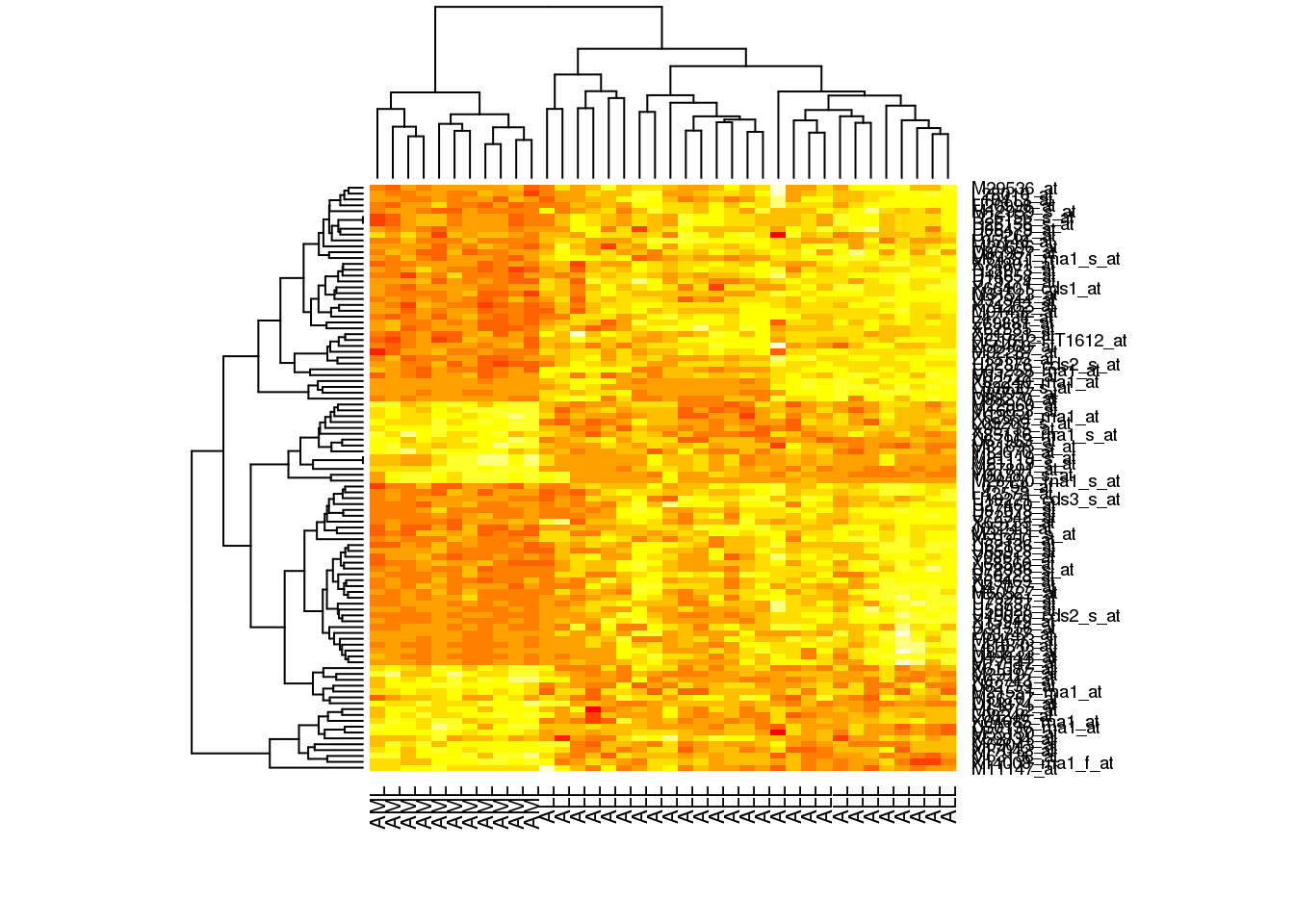
If we want to follow the conventional red-green microarray style, we can use the RdYlGn colour palette from the RColourBrewer package.
library(RColorBrewer)
heatmap(golub.100, col = brewer.pal(11, name='RdYlGn'))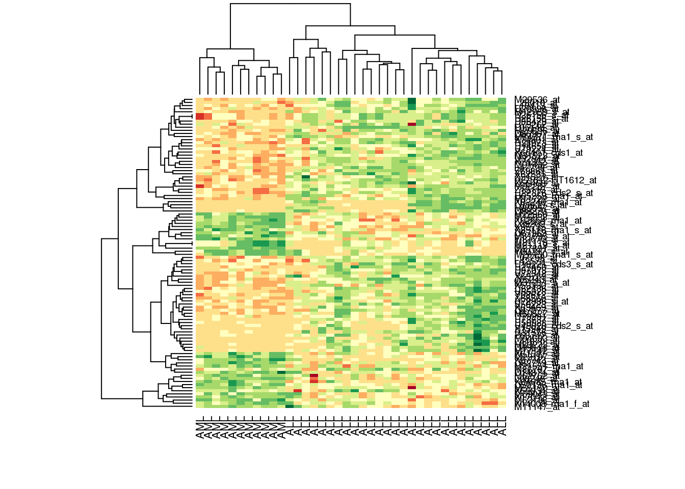
Use display.brewer.all() or display.brewer.pal(n,name) to see the range of palettes available from this package.
By default, this actually gives a very presentable plot. Both rows and columns are automatically sorted to cluster most alike genes and samples together, and dendrograms are plotted for us automatically. Encouragingly, we can see that all the \(AML\) and \(ALL\) samples form two separate clusters. It might look better without the crowded gene names column, but that can be turned off easily with the setting labRow = NA.
For more practice, see if you can prepare a heat plot of the Indometh dataset:
-
Hints:
- you will need to convert the dataset into a matrix with one column per Subject. Set column names as Subject number and rownames as timepoints
- review the Rowv setting to keep time points in order in the dendrogram
- think about transforming the data to compensate for the exponential decrease of the concentration value
- try different colour palettes to highlight the data
7.1.4 PCA plots
The final plotting option we will explore is principle component analysis, or PCA. PCA is often used where there are two or more categories of data, and multiple quantitative measurements on each, to quickly review whether the difference between the categories outweighs any noise or batch effect signals. Essentially, PCA collapses the dataset down to a small number of representative dimensions which can be plotted on a chart.
PCA analysis is widely used in expression datasets, which have large numbers of measurements (one per gene), multiple replicates, and normally two or more categorical conditions, so we will test it with our Golub dataset. We will use the PCA function of the ‘mixOmics’ package.
library(mixOmics)

# Carry out the PCA on just the top 100 genes, with default parameters
# N.B. PCA data needs to have the samples in rows. Our data is by
# columns, so we need to transpose it
golub.100.pca <- pca(t(golub.100))

# Then plot the data for the first two components, colouring the
# sample names for clarity
plotIndiv(golub.100.pca, comp = c(1,2),
          col = c(rep('red', 27), rep('blue', 11)))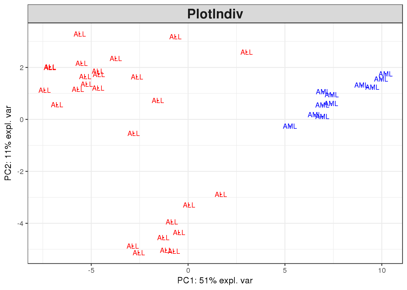
-
Generate a PCA plot for other components of the analysis
-
Carry out a PCA analysis for the full (normalised, transformed) Golub dataset and generate a plot
-
Does the data differentiate between the two sample types?