2.5 Understanding the dataset
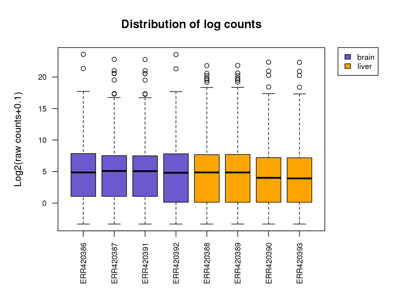
Density plots of log-intensity distribution of each library can be superposed on a single graph for a better comparison between libraries and for identification of libraries with weird distribution. On the boxplots the density distributions of raw log-intensities are not expected to be identical but still not totally different.
logcounts <- log2(raw.counts+0.1)

group.colours <- c('slateblue','orange')[group];
par(mar=c(5.1, 5, 4.1, 7), xpd=TRUE)
boxplot(logcounts,
        col=group.colours,
        main="Distribution of log counts",
        xlab="",
        ylab="Log2(raw counts+0.1)",
        las=2,cex.axis=0.8)
legend("topright", inset=c(-0.2,0), cex = 0.8,
       legend = levels(group),
       fill = unique(group.colours))