3.4 Importing from text files
Data is most commonly shared in tabular formats (Excel presents data in a tabular format). These are most-often text files that contain columns of data separated with comma, tab or other field-delimiters. In R there are some simple methods for quickly reading in massive amounts of data.
For the rest of this workshop we are going to work with a public dataset measuring the daily minimum and maximum temperatures across a number of cities in Australia. The data has been measured by 112 stations across Australia. The input file is located in folder: data/Intro_to_R/stations.txt.
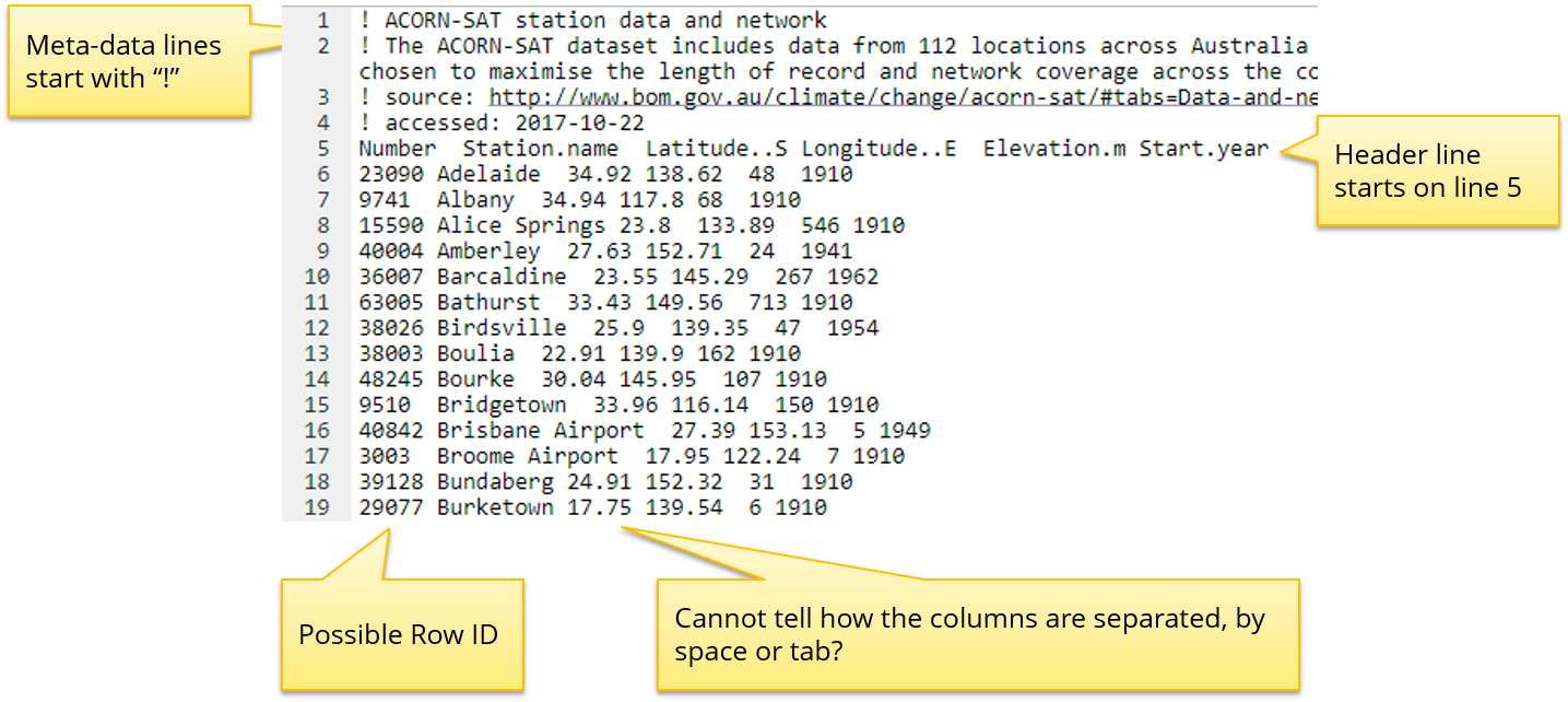
Stations.txt file
data.path <- "data/Intro_to_R"

# Of course, you will need a different path if the data is on your local P.C.
# e.g. data.path <- "C:/Intro_to_R/Data"
# Create a variable pointing to the file location.

stations.file <- file.path(data.path, "stations.txt")

# Then look at the start and finish of that file
head(readLines(stations.file))
tail(readLines(stations.file))
What is happening here?
| Function | Description |
|---|---|
readLines() |
reads each line from a target file into a vector. See also read.table, read.csv functions. |
file.path() |
DOES NOT read in the contents of a file. It just point to the location of a files on your system. You need to use readLines, read.table or similar to access the contents of that file. |
head() |
show first 6 lines of the object |
tail() |
show last 6 lines of object |
Using the head() and tail() commands helps us understand the nature of the file. It seems that the # prefix indicates metadata rather than data and the file is tab separated indicated by the ‘’ symbols.
Beware of printing large variables with RStudio Server, you can freeze your session. Judiciously use methods to limit the output:
- read into a variable first
- limit the output
-
use
head()/tail()functions
We have started to explore the contents of the expression data file using the code above, but at the moment have not imported it into a variable in R. The following exercise will step you through using the read.table() function in R to read a text file and import the data as a data.frame object.
When reading a table, R expects the same number of columns for every row, it will by default use the first line to determine the number of columns that are in your dataset. You can specify the separater to use depending on how your data columns are separated e.g. tab-delimited, comma-delimited or by something else altogether.
Reading in tabular data
-
Enter the previous code chunk to set up your
data.pathand take an initial look at the expression data in the variablestations.file. -
Open up the help documentation for
read.table()function while you perform the following worked example. Read up on the following parameters in detail:
-
sep -
comment -
header -
row.names
-
Follow the code below to use
read.table()to import the dataset into R. There should be 112 rows (stations) and 5 columns (variables), use the station number as the rownames since it will be unique.
Pay close attention to the dimension of the dataset after each read as each parameter will affect the read.
Attempt 1:: read.table using default settings:
This will fail because by default the sep parameter separates on white-space and the first X lines in the file are all comments, each line does not have the same number of columns as indicated by the error message.
stations <- read.table(stations.file)Error in scan(file = file, what = what, sep = sep, quote = quote, dec = dec, : line 1 did not have 42 elements
Attempt 2:: skip comment lines
We specify the separating delimiter (sep='\t'), the comment character (‘!’) and check the dimension of the data object after reading in the file. Is the number of rows and columns correct?
stations <- read.table(stations.file, comment.char = "!", sep='\t')
dim(stations)
## [1] 113 6We have 1 too many rows and columns. Taking a physical look a the object will tell us why. It is because we haven’t assigned the row or column names to the data frame.
head(stations)## V1 V2 V3 V4 V5 V6
## 1 Number Station.name Latitude..S Longitude..E Elevation.m Start.year
## 2 23090 Adelaide 34.92 138.62 48 1910
## 3 9741 Albany 34.94 117.8 68 1910
## 4 15590 Alice Springs 23.8 133.89 546 1910
## 5 40004 Amberley 27.63 152.71 24 1941
## 6 36007 Barcaldine 23.55 145.29 267 1962Attempt 3:: assign header and row names
stations <- read.table(stations.file, comment.char="!", sep="\t",
                       header=TRUE, row.names = 1)
dim(stations)
## [1] 112 5head(stations)## Station.name Latitude..S Longitude..E Elevation.m Start.year
## 23090 Adelaide 34.92 138.62 48 1910
## 9741 Albany 34.94 117.80 68 1910
## 15590 Alice Springs 23.80 133.89 546 1910
## 40004 Amberley 27.63 152.71 24 1941
## 36007 Barcaldine 23.55 145.29 267 1962
## 63005 Bathurst 33.43 149.56 713 1910Much better, this looks right!
Let’s save the stations variable as a Rdata object so that we don’t have to read it in again.
save(stations, file='stations.Rdata')Import temperature dataset
Now that you have imported the stations metadata, let’s import the actual temperatures for one station across the last 69 years.
Read in the minimum temperatures file: data/Intro_to_R/minTEmp.040842.csv into a variable named minTemp.
Use the first column (date) as the rownames, there should be 366 rows and 69 variables.
Expected output:
##       X1949 X1950 X1951 X1952 X1953
## Jan-1    NA  22.3  19.0  22.4  18.3
## Jan-2    NA  19.3  16.3  20.8  20.8
## Jan-3    NA  23.1  15.4  23.4  16.3
## Jan-4    NA  22.5  15.1  23.1  17.5
## Jan-5    NA  22.4  14.6  20.3  19.8
We will be working with this dataset in the following chapter.